The principles of input-output models are described briefly here. The essential feature is that the output of any industry is not entirely sold on a market for the industry’s product; some of it will be used by industries associated within the chain of production as an input for production; an example is the output of the sheet metal industry which will be in the large part purchased by motor vehicle and white goods manufacturers as input to the production of motor vehicles and refrigerators. More relevant local examples are the output of the agricultural industries, which provide inputs for the production of food and beverages, dairy production and support the manufacture of confectionary and dairy products; timber harvested by forest companies is sold to timber processors; while mining output is an input to the mineral processing industries. This backward and forward linking structure is an essential feature of an I/O table and defines its set of inter-industry relationships.

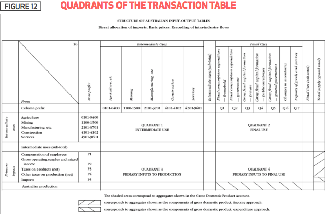
The development of an I/O model applied in this analysis is based on a transaction table developed by the ABS with the following structure:

• Each row shows the distribution of one industry to other industries and to final demand, while each column records the industry in questions’ acquisition of inputs from other industries in an economy. These are referred to as ‘intermediate purchases’ to distinguish them from final purchases/sales.
• The table contains four quadrants:
  • The processing sector is shown as Quadrant 1 and records the flow of goods and services between individual industries during a year.
  • The second quadrant records the consumption expenditures of final buyers and the other industry sectors from which they are made. A particular feature of Quadrant 2 is the presence of capital items which are included as part of the total expenditure of the individual industries, however, these capital goods are not used up for production in the current period and so they are shown for the production sector only.
  • Quadrant 3 records payments for the use of primary inputs in particular to labour (wages, recorded as Compensation Of Employees), to corporations as profits or rents (Gross Operating Surplus), to governments in various tiers as indirect taxes and charges and to importers. The value added by each industry to total national income, Gross Domestic or State Product measured at factor (input) cost is the combination of some of these payments as follows:

Value Added_i = WSS_i + GOS_i + Indirect taxes_i – subsidies_i

• So the value added by industry i is the sum of wages, salaries and supplements or compensation of employees (COE_i) paid to labour, the gross operating surplus (GOS_i) plus indirect taxes and charges net of subsidies paid by government to industry i. The sum of all the value added by the i industries constituting the economy is the value of Australia’s national income, namely GDP (Quadrant 4).

One of the objectives of the modelling is to determine how much GDP increases in response to the expenditure of an XXX project and in response to the increased expenditure by persons in response to XXX project, for example increased tourism.

In our analysis we also included an intermediary Table (with matrix identifier Z) which indicates the proportion of total supply of an industries output is met by a given industry. This is necessary due to the fact that sum industries produce goods that are measured as part of another sector (for example the ‘Other Industries’ sector producing service that are recorded as ‘Personal Services’). At this stage we also exclude the leakage associated with imports. This occurs when demand results in output of a particular sector being imported from overseas.

The Math of I/O Modelling

The transaction table may be presented in the following matrix form where X_ij is the amount of industry j’s output purchased by industry i as an input and D_i is the final demand for industry i’s output.

The transaction table above is defined by dividing the elements of the matrix above by the current value of industry i’s output. By this definition:

These a_ij are the technical coefficients of production and they represent the amount of industry i’s output required to produce a unit of output in industry j.

From (1) we can write:

and the output for industry i is the sum of intermediate sales and purchases plus the final demand for i’s output (D_i) as follows:

Where X is a vector of industry outputs, D is a vector of final demands and A is an i_xj matrix of technical coefficients.

The expression (3) can be solved for X as a function of D:

The solution vector represents the output of industries as some multiple of final demand (D) the multiple is the matrix (I-A)^-1=B. This is known as the Leontief inverse after its creator. Now B is structured in the following manner:

This is referred to as the table of interdependence coefficients and measures the direct, induced and indirect effects of a change in final demand for one of the industry outputs. The columns of this interdependence coefficient table are the output multipliers.

What do I/O output multipliers tell us? I/O output multipliers measure the changes in all industry outputs generated by a change in the final demand for any one output. For example, if the demand for agricultural output in Australia increased by 10%, then I/O output multipliers measure the impact on all industry output including agriculture.

Employment multipliers describe the impact of a change in the final demand for a specific industry’s output on employment in the same and all other industries. These I/O employment multipliers are derived from employment equations, which are derived in turn by simply multiplying the output equations for each industry by the employment (E_i)/Output (X₁) ratio for the industry in question. So the employment equation for industry 1 is found by multiplying (1) though by E_i/X₁. Then I/O employment multipliers are found in the same way by inverting the set of employment equations solving for employment in industry i.

Wage multipliers are found in an identical fashion, but on this occasion wage equations are employed to derive these. The wage multiplier measures the change in all industry wage incomes flowing from a change in any of the final demands.

However, there is also a wage-multiplier effect which effectively ‘closes’ the model with respect to the household sector. The wage-multiplier identifies the extent to which increased household income from wages raises expenditure in the community, thereby generating additional economic activity and employment. To incorporate the impact of increased wages on household final consumption expenditure (a component of final demand D) we derive a matrix C which is parallel to the matrix A. The element of matrix C, cij relate the expected increase in household final consumption expenditure associated with a unit increase in output by industry j.

Therefore final demand D contains a dependent component based on wages and an independent component that with identify as FD. We describe this relationship in equation [0.1].

The expression [1.5] can be substituted into [1.4] while maintaining the equality as follows:

The expression [1.6] can then be solved for equilibrium X = Y as a function of FD:

The solution vector B represent the output of industries as some multiple of final demand (FD) the multiple is the matrix . The structure of L is a table of interdependence coefficients and measures the direct, indirect and induced (where the model is closed) effects of a change in final demand for one of the industry outputs. The columns of this inter-dependence table are the output multipliers.

Output I/O multipliers measure the change in all industry outputs generated by a change in the final demand for any one output. Wage, value-added and employment multipliers are calculated based on the output multipliers. It is assumed that the relationship between output of a given sector and its wage, value-added and employment are constant (effectively determined by technology and structural parameters in the industry) so that if output in a sector increases by a given amount, then the value-added, wage and employment impacts can be calculated using a constant ratio for each industry.

Gross State Product (GSP) multipliers measure the contribution of a final demand change to each industry’s value added or its individual contribution to GSP. GSP multipliers are derived from total income equations which are output equations converted to total income relationships by applying value added/output ratios to each industry’s outputs.

All four sets of multipliers are applied to the task of identifying employment, GSP, wage and output effects of the XXXX project not proceeding.

Here, a distinction should be made between Type I and Type II multipliers. Type I income or output multipliers are the ratio of the direct plus indirect income or output change of demand to the direct income change resulting from a dollar increase in final demand for any given industry.

Type II multipliers are those derived mathematically above and can be read off the column of the B matrix in (7). In either case, type I or II, the I/O model is closed with respect to households which is the case here.

The practicality of I/O models depends on certain properties and assumptions. First, a workable I/O model will be mathematically stable which happens if the following holds:

The table of technical coefficients must have at least one column which sums to a number less than one. No column in the table can exceed one in the aggregate (no industry can pay more for its inputs than it receives from the sale of its output).

The following assumptions underpin all practical I/O models:

• A single production function exists for all firms in an industry.
• This production function must be linear and be homogeneous of degree I (Constant Returns to scale applies).
• There is no substitutability between factions of production (labour and capital).